Database Internal - B-tree Summary

• The B-tree basic in database system.

• The B-tree basic in database system.
• Here is the basic of B-tree, including the knowledge of data structure and some optimization.
• The content is based on the book Database Internal and Algorithms Visualization.I will present my understanding.
• Only summary, not details.

Before B-Tree

The B-tree is usually used for index of data. I want to introduce a simple data structure which is used in simple query operation.

• Sorted List: If data is sorted, we can look up the data quickly. Two major methods: (Eg. Look up 12)
  • Linear Search: From the start/end of the list, compare the data with target data 12 one by one.
    • Time complexity: $O(N)$
  • Binray Search: Get the max, min, and middle data of this sorted list by reading the data with given index (0, list.length and list.length / 2). Compare these data with target data to find the target data located area. In small area, recurse until find the target data or mark it not found.
    • Time complexity: $O(\log_2{Nx })$

B-Tree

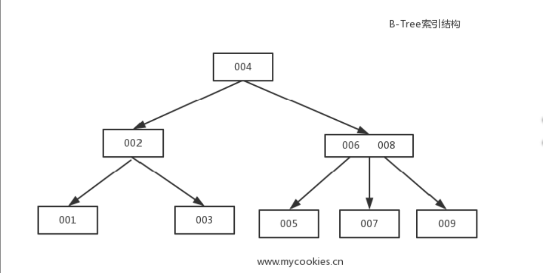
• B-Tree was introduced by Rudolph Bayer and Edward M. McCreight back in 1971.

Binary Search Tree (BST)

• Sorted, In-Memory data structure.
• Used for efficient key-value lookups.
• Represented by a key, a value associated with this key.
• Each node splits the search space into left and right subtrees, as figure shows: a node key is greater than any key stored in its left subtree and less than any key stored in its right subtree.
  
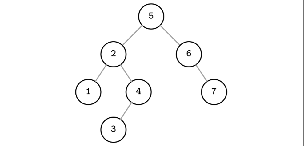
• Look up from root node, if greater than root node, try to look up in the right child tree. If less, continue to look up in left child tree. Recurse until find it or compared all leaf nodes.

Tree Balancing

Why need balancing ?

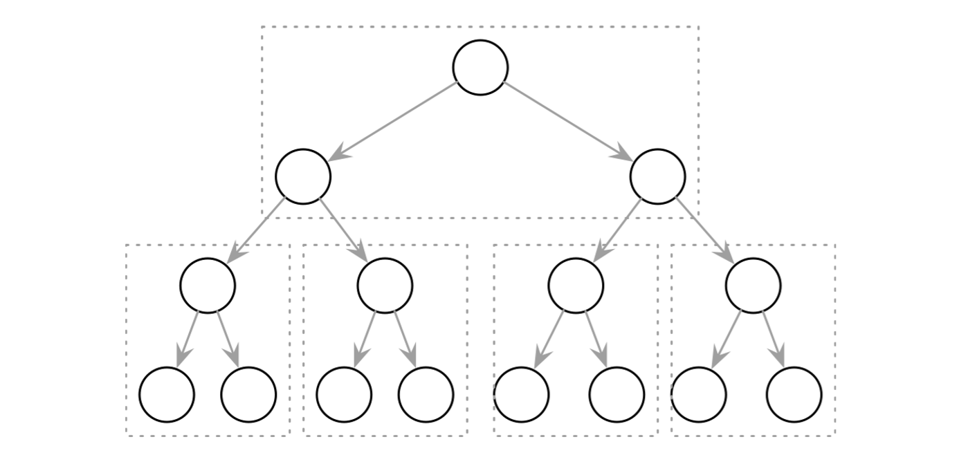
• Insert operations do not follow any specific pattern, and element insertion might lead to the situation where the tree is unbalanced (i.e., one of its branches is longer than the other one).
• The worst-case scenario is shown in Figure (b), where we end up with a pathological tree, which looks more like a linked list, and instead of desired logarithmic complexity, we get linear, as illustrated in Figure (a).
  
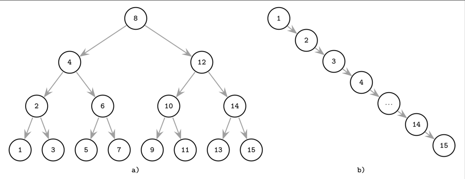
• In the balanced tree, following the left or right node pointer reduces the search space in half on average, so lookup complexity is logarithmic: $O(\log_2{N})$. If the tree is not balanced, worst-case complexity goes up to $O(N)$, since we might end up in the situation where all elements end up on one side of the tree.

How to balance?

• Balance Status: Balancing is done by reorganizing nodes in a way that minimizes tree height and keeps the number of nodes on each side within bounds.
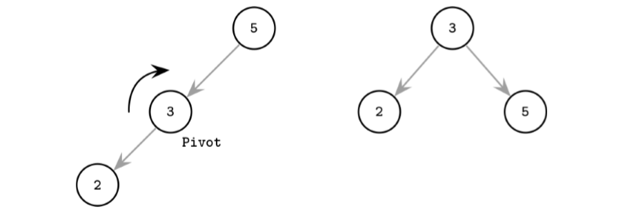
• One of the ways to keep the tree balanced is to perform a rotation step after nodes are added or removed. If the insert operation leaves a branch unbalanced (two consecutive nodes in the branch have only one child), we can rotate nodes around the middle one.
• In the example shown in Figure 2-4, during rotation the middle node (3), known as a rotation pivot, is promoted one level higher, and its parent becomes its right child.
  

Trees for Disk-Based Storage

• As previously mentioned, unbalanced trees have a worst-case complexity of $O(N)$. Balanced trees give us an average $O(\log_2{N})$.
• At the same time, due to low fanout (fanout is the maximum allowed number of children per node), we have to perform balancing, relocate nodes, and update pointers rather frequently. Increased maintenance costs make BSTs impractical as on-disk data structures.

Problems

• Locality: since elements are added in random order, there’s no guarantee that a newly created node is written close to its parent, which means that node child pointers may span across several disk pages.
  • We can improve the situation to a certain extent by modifying the tree layout and using paged binary trees.
• Tree height: Since binary trees have a fanout of just two, height is a binary logarithm of the number of the elements in the tree, and we have to perform $O(\log_2{N})$ seeks to locate the searched element and, subsequently, perform the same number of disk transfers.
  • 2-3 Trees and other low-fanout trees have a similar limitation: while they are useful as in-memory data structures, small node size makes them impractical for external storage.
  • A naive on-disk BST implementation would require as many disk seeks as comparisons, since there’s no built-in concept of locality. This sets us on a course to look for a data structure that would exhibit this property.

Requirements

• High fanout to improve locality of the neighboring keys.
• Low height to reduce the number of seeks during traversal.
• Fanout and height are inversely correlated.

Disk-Based Structures

• On-disk data structures are often used when the amounts of data are so large that keeping an entire dataset in memory is impossible or not feasible. Only a fraction of the data can be cached in memory at any time, and the rest has to be stored on disk in a manner that allows efficiently accessing it.

Hard Disk Drives

• On spinning disks, seeks increase costs of random reads because they require disk rotation and mechanical head movements to position the read/write head to the desired location. However, once the expensive part is done, reading or writing contiguous bytes (i.e., sequential operations) is relatively cheap.
• The smallest transfer unit of a spinning drive is a sector, so when some operation is performed, at least an entire sector can be read or written. Sector sizes typically range from 512 bytes to 4 Kb.
• Head positioning is the most expensive part of an operation on the HDD. This is one of the reasons we often hear about the positive effects of sequential I/O: reading and writing contiguous memory segments from disk.
• Benefit a lot from the performance gap between sequential I/O and random I/O.

Solid State Drives

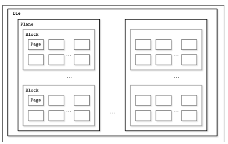
• A typical SSD is built of memory cells, connected into strings (typically 32 to 64 cells per string), strings are combined into arrays, arrays are combined into pages, and pages are combined into blocks.
• Depending on the exact technology used, a cell can hold one or multiple bits of data. Pages vary in size between devices, but typically their sizes range from 2 to 16 Kb. Blocks typically contain 64 to 512 pages. Blocks are organized into planes and, finally, planes are placed on a die. SSDs can have one or more dies. You can view the details of SSD structure from this post Virtual SSD
  
• Since in both device types (HDDs and SSDs) we are addressing chunks of memory rather than individual bytes (i.e., accessing data block-wise), most operating systems have a block device abstraction. It hides an internal disk structure and buffers I/O operations internally, so when we’re reading a single word from a block device, the whole block containing it is read. This is a constraint we cannot ignore and should always take into account when working with disk-resident data structures.
• In SSDs, we don’t have a strong emphasis on random versus sequential I/O, as in HDDs, because the difference in latencies between random and sequential reads is not as large. There is still some difference caused by prefetching, reading contiguous pages, and internal parallelism.
• Even though garbage collection is usually a background operation, its effects may negatively impact write performance, especially in cases of random and unaligned write workloads.
• Writing only full blocks, and combining subsequent writes to the same block, can help to reduce the number of required I/O operations.

On-Disk Structures

Limitations

• The cost of disk access itself.
• Major: The smallest unit of disk operation is a block.

Ideas

• On-disk structures are designed with their target storage specifics in mind and generally optimize for fewer disk accesses. We can do this by improving locality, optimizing the internal representation of the structure, and reducing the number of out-of-page pointers.
• From above chapters, we came to the conclusion that high fanout and low height are desired properties for an optimal on-disk data structure. We’ve also just discussed additional space overhead coming from pointers, and maintenance overhead from remapping these pointers as a result of balancing.
• B-Trees combine these ideas:
  • increase node fanout
  • reduce tree height
  • the number of node pointers
  • the frequency of balancing operations.

Paged Binary Trees

Laying out a binary tree by grouping nodes into pages

• Improves the situation with locality. To find the next node, it’s only necessary to follow a pointer in an already fetched page.
• However, there’s still some overhead incurred by the nodes and pointers between them. Laying the structure out on disk and its further maintenance are nontrivial endeavors, especially if keys and values are not presorted and added in random order. Balancing requires page reorganization, which in turn causes pointer updates.

Ubiquitous B-Trees

• B-Tree is not Binary Tree. It means Balanced Tree.
• B-Tree builds a hierarchy that helps to navigate and locate the searched items quickly.
• B-Trees build upon the foundation of balanced search trees and are different in that they have higher fanout (have more child nodes) and smaller height.
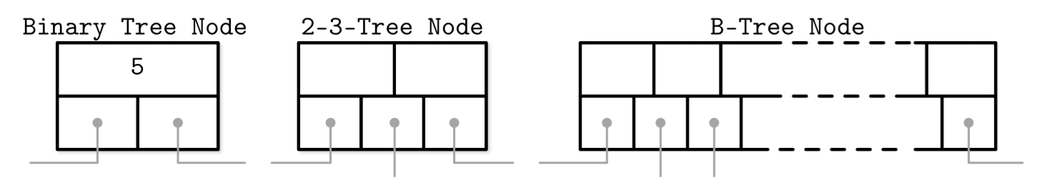
• Differences with binary trees:
  • binary tree nodes are drawn as circles. Since each node is responsible just for one key and splits the range into two parts
  • B-Tree nodes are often drawn as rectangles, and pointer blocks are also shown explicitly to highlight the relationship between child nodes and separator keys.

• If we use same way to depicte binary tree, and it will look like as follows:
  
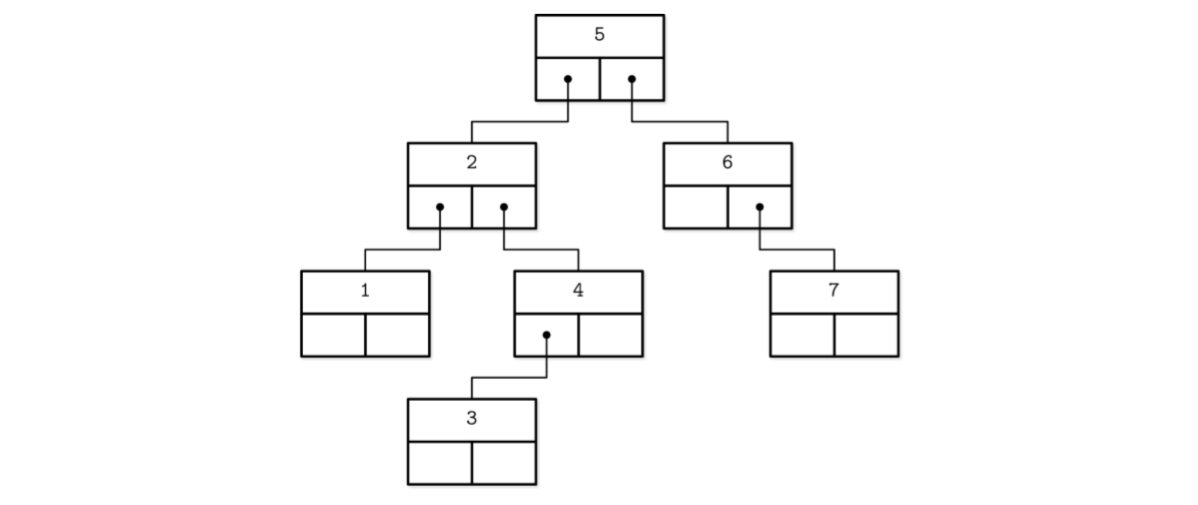
• B-Trees are sorted: keys inside the B-Tree nodes are stored in order.
  • Because of that, to locate a searched key, we can use an algorithm like binary search. This also implies that lookups in B-Trees have logarithmic complexity.
  • Since B-Tree nodes store dozens or even hundreds of items, we only have to make one disk seek per level jump.
• Using B-Trees, we can efficiently execute both point and range queries.

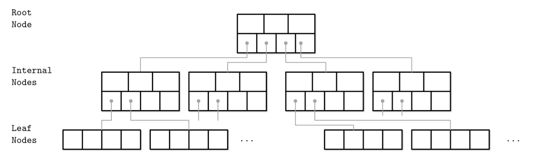
B-Tree Hierarchy

Components

• B-Trees consist of multiple nodes.
  • Each node holds up to N keys and N + 1 pointers to the child nodes.
• These nodes are logically grouped into three groups:
  • Root node
  • Leaf nodes
  • Internal nodes

Concepts

• Since B-Trees are a page organization technique (i.e., they are used to organize and navigate fixed-size pages), we often use terms node and page interchangeably.
• The relation between the node capacity and the number of keys it actually holds is called occupancy.
• fanout: the number of keys stored in each node.
  • Higher fanout helps to amortize the cost of structural changes required to keep the tree balanced and to reduce the number of seeks by storing keys and pointers to child nodes in a single block or multiple consecutive blocks.
• Balancing operations (namely, splits and merges) are triggered when the nodes are full or nearly empty.

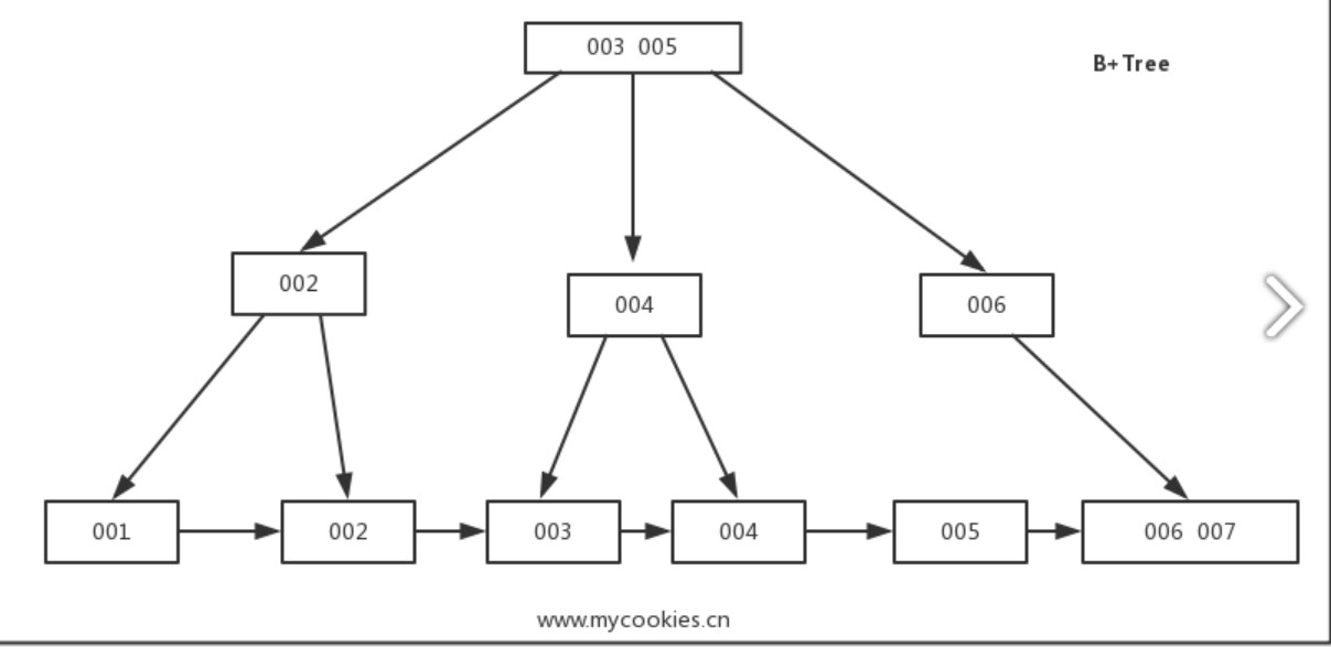
B+ Trees

• B-Trees allow storing values on any level: in root, internal, and leaf nodes. B+-Trees store values only in leaf nodes.
• Internal nodes store only separator keys used to guide the search algorithm to the associated value stored on the leaf level.
• Since values in B+-Trees are stored only on the leaf level, all operations (inserting, updating, removing, and retrieving data records) affect only leaf nodes and propagate to higher levels only during splits and merges.
• $B^+$ Tree is used in MySQL index. You can view the details about differences between B+ tree and B-tree by clicking https://www.cnblogs.com/liqiangchn/p/9060521.html.

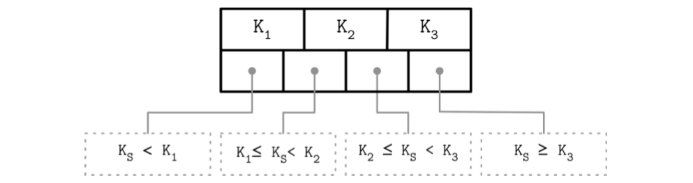
Separator Keys

• Keys stored in B-Tree nodes are called index entries, separator keys, or divider cells. They split the tree into subtrees (also called branches or subranges), holding corresponding key ranges. Keys are stored in sorted order to allow binary search. A subtree is found by locating a key and following a corresponding pointer from the higher to the lower level.

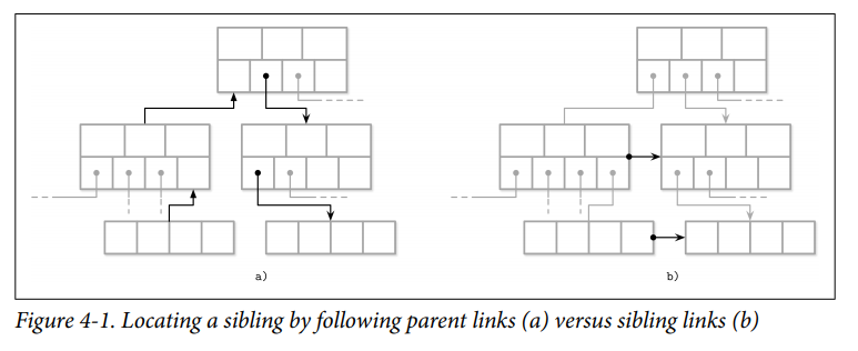
• Some B-Tree variants also have sibling node pointers, most often on the leaf level, to simplify range scans。(Such as B+ tree)
  • These pointers help avoid going back to the parent to find the next sibling.
  • Some implementations have pointers in both directions, forming a double-linked list on the leaf level, which makes the reverse iteration possible.
• Storage Utilization: Since B-Trees reserve extra space inside nodes for future insertions and updates, tree storage utilization can get as low as 50%, but is usually considerably higher. Higher occupancy does not influence B-Tree performance negatively.

How to build B-Tree?

• What sets B-Trees apart is that, rather than being built from top to bottom (as binary search trees), they’re constructed the other way around—from bottom to top. The number of leaf nodes grows, which increases the number of internal nodes and tree height.

B-Tree Lookup Complexity

• 2 standpoints:
  • the number of block transfers
  • the number of comparisons done during the lookup

Block transfers

• Assume number of keys per node is N; K times more nodes on each new level; M is a total number of items in the B-Tree.
• To find a searched key, at most $\log_K{M}$ pages are addressed.

Comparisons done during the lookup

• From the perspective of number of comparisons, the logarithm base is 2, since searching a key inside each node is done using binary search. Every comparison halves the search space, so complexity is $\log_2 M$.

B-Tree Lookup Algorithm

• To find an item in a B-Tree, we have to perform a single traversal from root to leaf. The objective of this search is to find a searched key or its predecessor.
  • Finding an exact match is used for point queries, updates, and deletions
  • Finding its predecessor is useful for range scans and inserts.
• The algorithm starts from the root and performs a binary search, comparing the searched key with the keys stored in the root node until it finds the first separator key that is greater than the searched value. This locates a searched subtree.
• As soon as we find the subtree, we follow the pointer that corresponds to it and continue the same search process (locate the separator key, follow the pointer) until we reach a target leaf node, where we either find the searched key or conclude it is not present by locating its predecessor.
  • During the point query, the search is done after finding or failing to find the searched key.
  • During the range scan, iteration starts from the closest found key-value pair and continues by following sibling pointers until the end of the range is reached or the range predicate is exhausted.

Couting Keys

B-Tree Node Splits

• To insert the value into a B-Tree, we first have to locate the target leaf and find the insertion point. For that, we use the algorithm described in the previous section. After the leaf is located, the key and value are appended to it.

• Updates in B-Trees work by locating a target leaf node using a lookup algorithm and associating a new value with an existing key.

• If the target node doesn’t have enough room available, we say that the node has overflowed and has to be split in two to fit the new data. Split conditions:

  • For leaf nodes: if the node can hold up to N key-value pairs, and inserting one more key-value pair brings it over its maximum capacity N.
  • For nonleaf nodes: if the node can hold up to N + 1 pointers, and inserting one more pointer brings it over its maximum capacity N + 1.

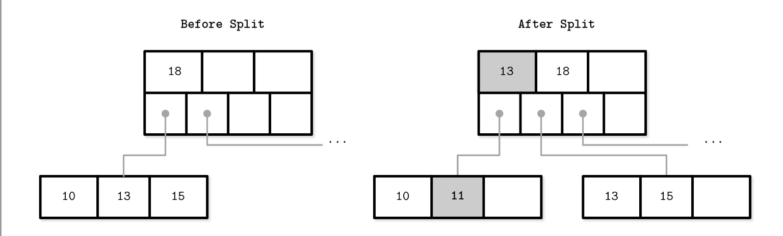
• Splits are done by allocating the new node, transferring half the elements from the splitting node to it, and adding its first key and pointer to the parent node. In this case, we say that the key is promoted. The index at which the split is performed is called the split point (also called the midpoint).

  • All elements after the split point (including split point in the case of nonleaf node split) are transferred to the newly created sibling node.
  • The rest of the elements remain in the splitting node.
  • If the parent node is full and does not have space available for the promoted key and pointer to the newly created node, it has to be split as well. This operation might propagate recursively all the way to the root.
    • As soon as the tree reaches its capacity (i.e., split propagates all the way up to the root), we have to split the root node.
    • When the root node is split, a new root, holding a split point key, is allocated. The old root (now holding only half the entries) is demoted to the next level along with its newly created sibling, increasing the tree height by one.
  • The tree height change conditions:
    • the root node is split and the new root is allocated
    • two nodes are merged to form a new root
  • On the leaf and internal node levels, the tree only grows horizontally.

• i.e. Leaf node split during the insertion of 11. New element and promoted key are shown in gray.
  

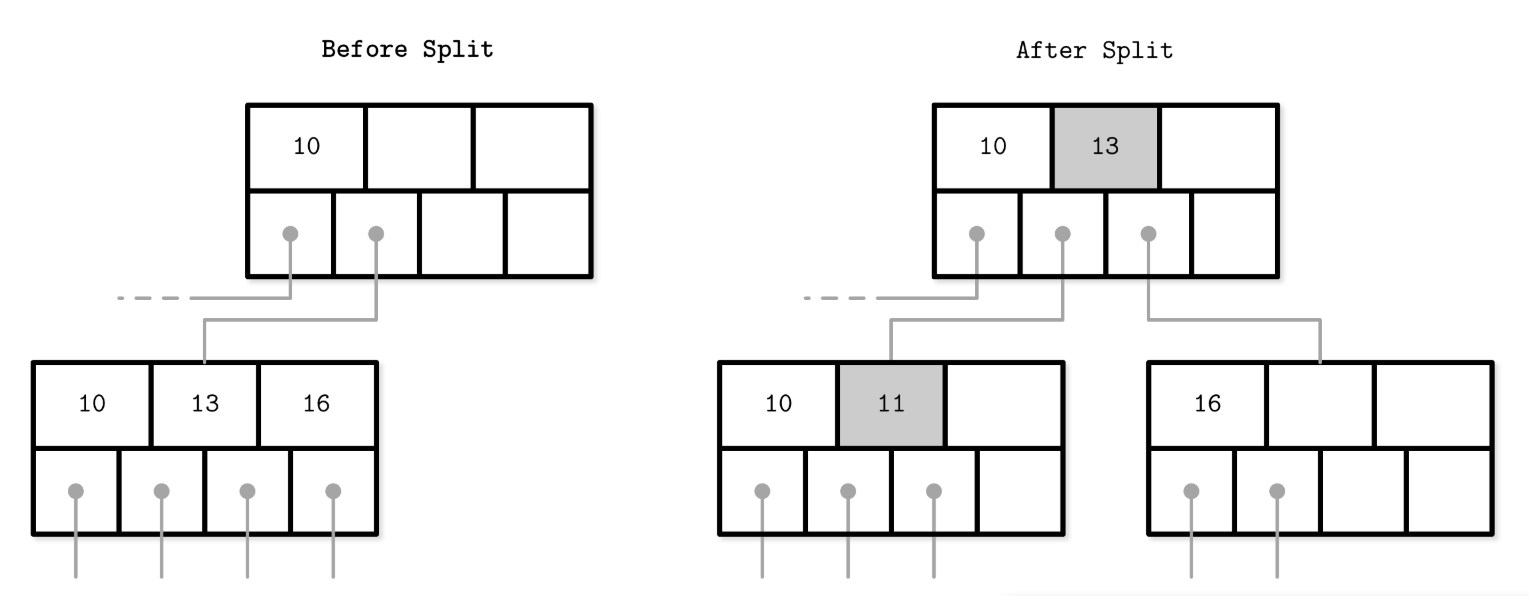
• i.e. Nonleaf node split during the insertion of 11. New element and promoted key are shown in gray.
  

Steps

1. Allocate a new node.
2. Copy half the elements from the splitting node to the new one.
3. Place the new element into the corresponding node.
4. At the parent of the split node, add a separator key and a pointer to the new node.

B-Tree Node Merges

If neighboring nodes have too few values (i.e., their occupancy falls under a threshold), the sibling nodes are merged. This situation is called underflow.

• It may need to merge nodes when delete elements.

Merge Conditions

• For leaf nodes: if a node can hold up to N key-value pairs, and a combined number of key-value pairs in two neighboring nodes is less than or equal to N.
• For nonleaf nodes: if a node can hold up to N + 1 pointers, and a combined number of pointers in two neighboring nodes is less than or equal to N + 1.

How to merge nodes

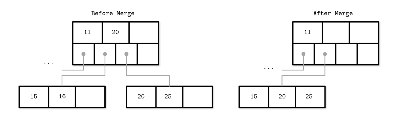
• i.e. DELETE 16 - Leaf node merge: Generally, elements from the right sibling are moved to the left one, but it can be done the other way around as long as the key order is preserved.
  
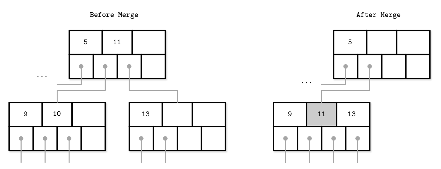
• i.e. DELETE 10 - Nonleaf node merge: During the merge of nonleaf nodes, we have to pull the corresponding separator key from the parent (i.e., demote it). The number of pointers is reduced by one because the merge is a result of the propagation of the pointer deletion from the lower level, caused by the page removal. Just as with splits, merges can propagate all the way to the root level.
  

Steps

1. Copy all elements from the right node to the left one.
2. Remove the right node pointer from the parent (or demote it in the case of a nonleaf merge).
3. Remove the right node.

Summary

• Binary search trees might have similar complexity characteristics, but still fall short of being suitable for disk because of low fanout and a large number of relocations and pointer updates caused by balancing.
• B-Trees solve both problems by increasing the number of items stored in each node (high fanout) and less frequent balancing operations.
• We can use this knowledge to create in-memory B-Trees. To create a disk-based implementation, we need to go into details of how to lay out B-Tree nodes on disk and compose on-disk layout using data-encoding formats.

File Formats

Explore how exactly B-Trees and other structures are implemented on disk.

• We access the disk in a way that is different from how we access main memory.
  • From an application developer’s perspective, memory accesses are mostly transparent. Because we do not have to manage virtual memory offsets manually.
  • Disks are accessed using system calls. We usually have to specify the offset inside the target file, and then interpret on-disk representation into a form suitable for main memory.
• The semantics of pointer management in on-disk structures are somewhat different from in-memory ones. It is useful to think of on-disk B-Trees as a page management mechanism: algorithms have to compose and navigate pages. Pages and pointers to them have to be calculated and placed accordingly.

Motivation

• The differences between memory and disks when we program with:
  • Memory: Unmanaged memory model.
    • We allocate a block of data and slice it any way we like, using fixed-size primitives and structures. If we want to reference a larger chunk of memory or a structure with variable size, we use pointers.
    • We can allocate more memory any time we need (within reasonable bounds) without us having to think or worry about whether or not there’s a contiguous memory segment available, whether or not it is fragmented, or what happens after we free it.
  • Disk: We have to take care of garbage collection and fragmentation ourselves.
    • For a disk-resident data structure to be efficient, we need to lay out data on disk in ways that allow quick access to it, and consider the specifics of a persistent storage medium, come up with binary data formats, and find a means to serialize and deserialize data efficiently.
• Even though the operating system and filesystem take over some of the responsibilities, implementing on-disk structures requires attention to more details and has more pitfalls.

Binary Encoding

• To store data on disk efficiently, it needs to be encoded using a format that is compact and easy to serialize and deserialize.
• Since we do not have primitives such as malloc and free, but only read and write, we have to think of accesses differently and prepare data accordingly.
• Before we can organize records into pages, we need to understand how to represent keys and data records in binary form, how to combine multiple values into more complex structures, and how to implement variable-size types and arrays

Primitive Types

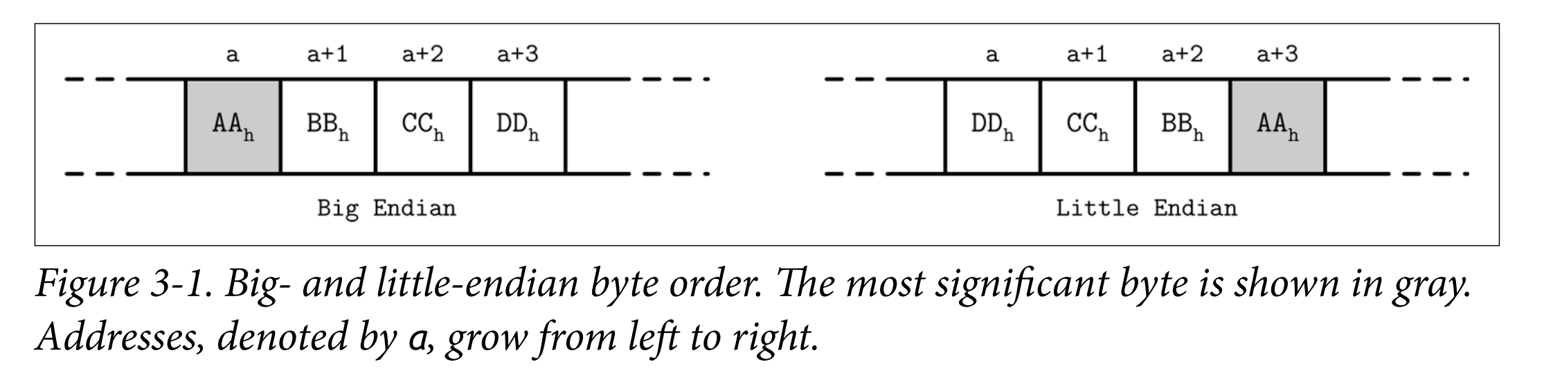
• Most numeric data types are represented as fixed-size values. When working with multibyte numeric values, it is important to use the same byte-order (endianness) for both encoding and decoding. Endianness determines the sequential order of bytes:
  • Big-endian: The order starts from the most-significant byte (MSB), followed by the bytes in decreasing significance order. In other words, MSB has the lowest address.
  • Little-endian: The order starts from the least-significant byte (LSB), followed by the bytes in increasing significance order.
    
• Records consist of primitives like numbers, strings, booleans, and their combinations. However, when transferring data over the network or storing it on disk, we can only use byte sequences.
  • In order to send or write the record, we have to serialize it (convert it to an interpretable sequence of bytes)
  • Before we can use it after receiving or reading, we have to deserialize it (translate the sequence of bytes back to the original record).

Number

• Different numeric types may vary in size.
  • byte value is 8 bits
  • short is 2 bytes (16 bits)
  • int is 4 bytes (32 bits)
  • long is 8 bytes (64 bits)
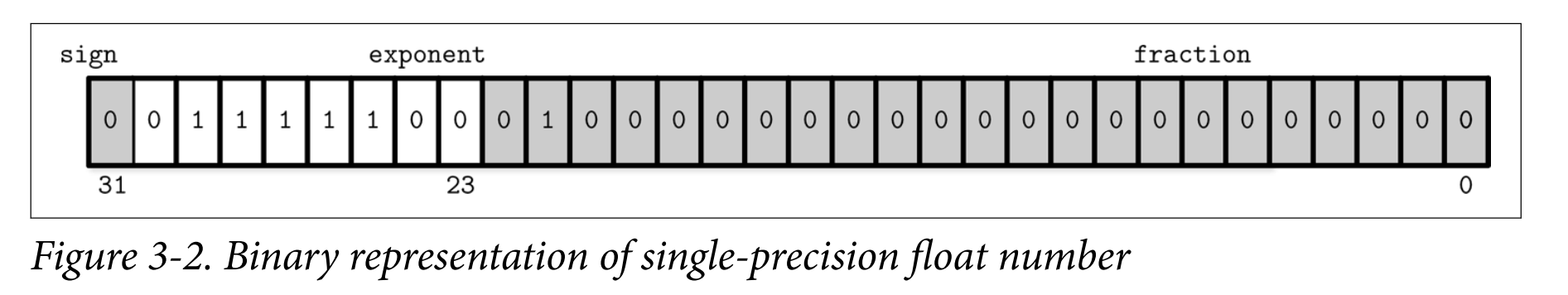
• Floating-point numbers (such as float and double) are represented by their sign, fraction, and exponent.
  • IEEE 754 Standard: A 32-bit float represents a single-precision value.
  • For example, a floating-point number 0.15652 has a binary representation, as shown in Figure 3-2. 计算机基础——IEEE754标准的浮点数的转化
    • The first 23 bits represent a fraction
    • The following 8 bits represent an exponent
    • 1 bit represents a sign (whether or not the number is negative).
      
• The double represents a double-precision floating-point value.

Strings and Variable-Size Data

• Composing more complex values together is much like struct
  in C. You can combine primitive values into structures and use fixed-size arrays or pointers to other memory regions.
• Strings and other variable-size data types (such as arrays of fixed-size data) can be serialized as a number, representing the length of the array or string, followed by size bytes: the actual data.
• For strings, this representation is often called UCSD String or Pascal String, named after the popular implementation of the Pascal programming language.

String 
{
  size   uint_16; 
  data   byte[size];
}

Bit-Packed Data: Booleans, Enums, and Flags

• Booleans can be represented either by using a single byte, or encoding true and false as 1 and 0 values.
• Enums, short for enumerated types, can be represented as integers and are often used in binary formats and communication protocols. Enums are used to represent oftenrepeated low-cardinality values.

enum NodeType { 
  ROOT,     // 0x00h
  INTERNAL, // 0x01h 
  LEAF      // 0x02h 
};

• Flags, kind of a combination of packed booleans and enums. Flags can represent nonmutually exclusive named boolean parameters.

int IS_LEAF_MASK = 0x01h; // bit #1
int VARIABLE_SIZE_VALUES = 0x02h; // bit #2 
int HAS_OVERFLOW_PAGES = 0x04h; // bit #3

• Just like packed booleans, flag values can be read and written from the packed value using bitmasks and bitwise operators.

// Set the bit
flags |= HAS_OVERFLOW_PAGES; 
flags |= (1 << 2);

// Unset the bit
flags &= ~HAS_OVERFLOW_PAGES; 
flags &= ~(1 << 2);

// Test whether or not the bit 
is set is_set = (flags & HAS_OVERFLOW_PAGES) != 0; 
is_set = (flags & (1 << 2)) != 0;

General Principles

• How the addressing is going to be done
  • Whether the file is going to be split into same-sized pages, which are represented by a single block or multiple contiguous blocks.
  • Most in-place update storage structures use pages of the same size, since it significantly simplifies read and write access.
  • Append-only storage structures often write data page-wise, too: records are appended one after the other and, as soon as the page fills up in memory, it is flushed on disk.
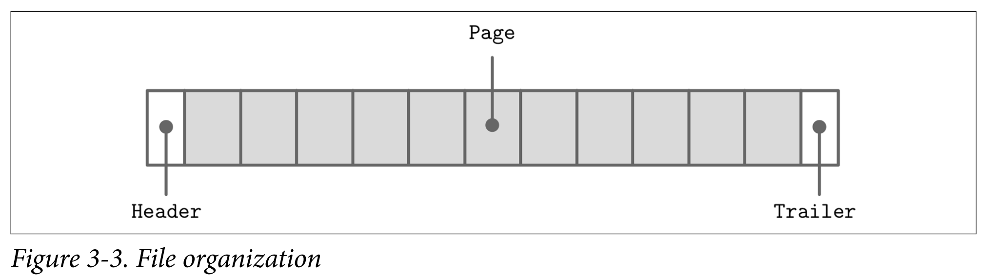
• The file usually starts with a fixed-size header and may end with a fixed-size trailer, which hold auxiliary information that should be accessed quickly or is required for decoding the rest of the file.
  
• Many data stores have a fixed schema, specifying the number, order, and type of fields the table can hold. Having a fixed schema helps to reduce the amount of data stored on disk: instead of repeatedly writing field names, we can use their positional identifiers. It is similar to relation database.
  • ex. Company Employee.
    
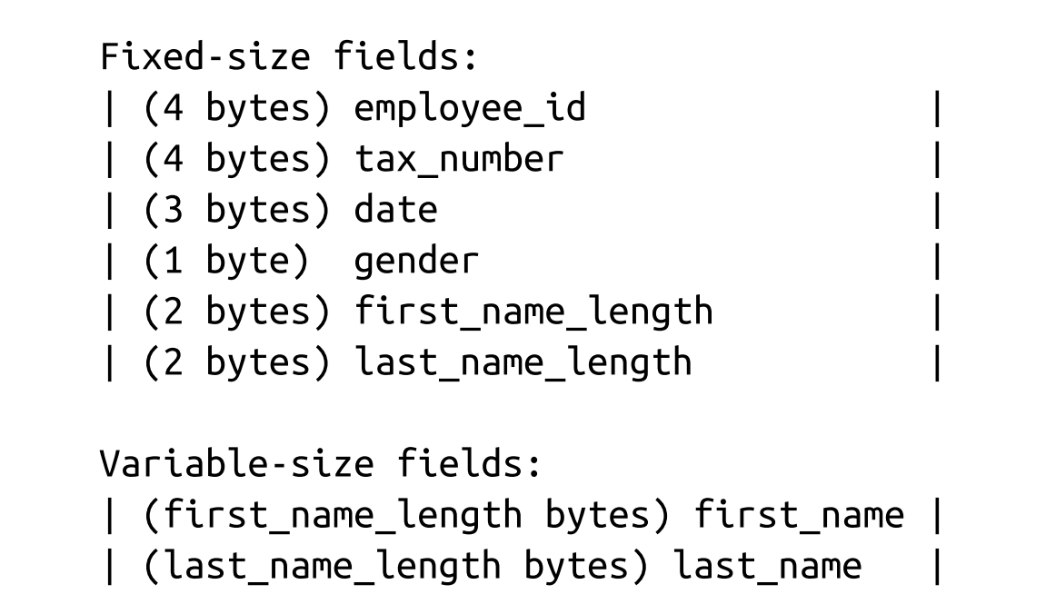
  • Now, to access first_name, we can slice first_name_length bytes after the fixed-size area. To access last_name, we can locate its starting position by checking the sizes of the variable-size fields that precede it.
  • To avoid calculations involving multiple fields, we can encode both offset and length to the fixed-size area. In this case, we can locate any variable-size field separately.
• Database files often consist of multiple parts, with a lookup table aiding navigation and pointing to the start offsets of these parts written either in the file header, trailer, or in the separate file.

Page Structure

• Database systems store data records in data and index files. These files are partitioned into fixed-size units called pages, which often have a size of multiple filesystem blocks. Page sizes usually range from 4 to 16 Kb.
• The original B-Tree paper [BAYER72] describes a simple page organization for fixedsize data records, where each page is just a concatenation of triplets, as shown in Figure 3-4: keys are denoted by k, associated values are denoted by v, and pointers to child pages are denoted by p.
  
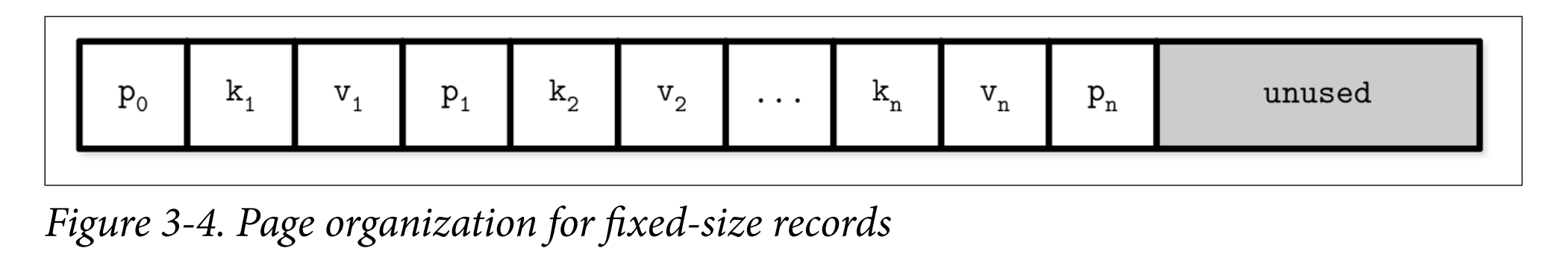
• Some downsides:
  • Appending a key anywhere but the right side requires relocating elements
  • It doesn’t allow managing or accessing variable-size records efficiently and works only for fixed-size data.

Slotted Pages

• When storing variable-size records, the main problem is free space management: reclaiming the space occupied by removed records.\
• To simplify space management for variable-size records, we can split the page into fixed-size segments. However, we end up wasting space if we do that, too.
  • For example, if we use a segment size of 64 bytes, unless the record size is a multiple of 64, we waste 64 - (n modulo 64) bytes, where n is the size of the inserted record. In other words, unless the record is a multiple of 64, one of the blocks will be only partially filled.
• Space reclamation can be done by simply rewriting the page and moving the records around, but we need to preserve record offsets, since out-of-page pointers might be using these offsets.

Goal

• Store variable-size records with a minimal overhead.
• Reclaim space occupied by the removed records.
• Reference records in the page without regard to their exact locations.

Slotted Page

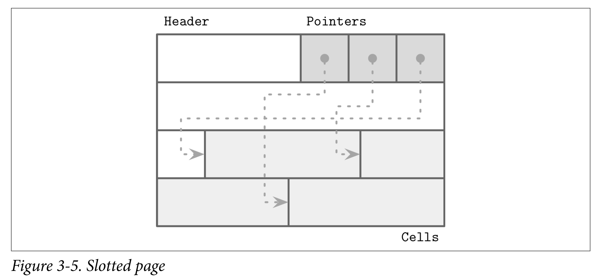
• To efficiently store variable-size records such as strings, binary large objects (BLOBs), etc., we can use an organization technique called slotted page. Used in PostgreSQL.
• We organize the page into a collection of slots or cells and split out pointers and cells in two independent memory regions residing on different sides of the page.
• A slotted page has a fixed-size header that holds important information about the page and cells. Cells may differ in size and can hold arbitrary data: keys, pointers, data records, etc. Figure 3-5 shows a slotted page organization, where every page has a maintenance region (header), cells, and pointers to them.
  
• How to achieve the goal?
  • Minimal overhead: the only overhead incurred by slotted pages is a pointer array holding offsets to the exact positions where the records are stored.
  • Space reclamation: space can be reclaimed by defragmenting and rewriting the page.
  • Dynamic layout: from outside the page, slots are referenced only by their IDs, so the exact location is internal to the page.

Cell Layout

• On a cell level, we have a distinction between key and key-value cells.
  • Key cells hold a separator key and a pointer to the page between two neighboring pointers.
  • Key-value cells hold keys and data records associated with them.
• We assume that all cells within the page are uniform (for example, all cells can hold either just keys or both keys and values; similarly, all cells hold either fixed-size or variable-size data, but not a mix of both). This means we can store metadata describing cells once on the page level, instead of duplicating it in every cell.

Key Cell

• To compose a key cell, we need to know:
  • Cell type (can be inferred from the page metadata)
  • Key size
  • ID of the child page this cell is pointing to
  • Key bytes
• A variable-size key cell layout might look something like this (a fixed-size one would have no size specifier on the cell level:

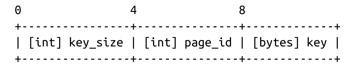
• We have grouped fixed-size data fields together, followed by key_size bytes. With Fixed Size key, the offset is easy to be calculated by using static and precomputed offsets. For Variable size key, we need to use the key_size for every key offset calculation.

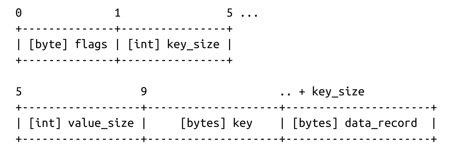
Key-Value Cells

• The key-value cells hold data records instead of the child page IDs.
  • Cell type (can be inferred from page metadata)
  • Key size
  • Value size
  • Key bytes
  • Data record bytes *

Combining Cells into Slotted Pages

• We append cells to the right side of the page (toward
  its end) and keep cell offsets/pointers in the left side of the page, as shown in Figure 3-6.

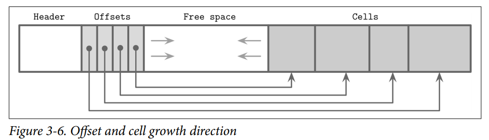
• Keys can be inserted out of order and their logical sorted order is kept by sorting cell offset pointers in key order. This design allows appending cells to the page with minimal effort, since cells don’t have to be relocated during insert, update, or delete operations.
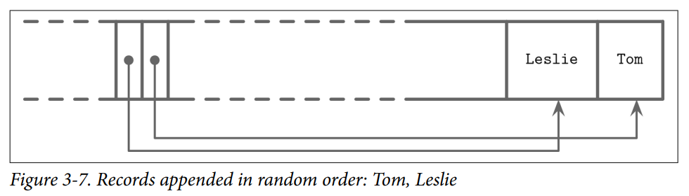
  • ex. Two names are added to thepage, and their insertion order is: Tom and Leslie. As you can see in Figure 3-7, their logical order (in this case, alphabetical), does not match insertion order (order in which they were appended to the page). Cells are laid out in insertion order, but offsets are re-sorted to allow using binary search.
    
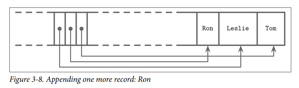
  • Now, we’d like to add one more name to this page: Ron. New data is appended at the upper boundary of the free space of the page, but cell offsets have to preserve the lexi‐cographical key order: Leslie, Ron, Tom. To do that, we have to reorder cell offsets: pointers after the insertion point are shifted to the right to make space for the new pointer to the Ron cell, as you can see in Figure 3-8.
    

Managing Variable-Size Data

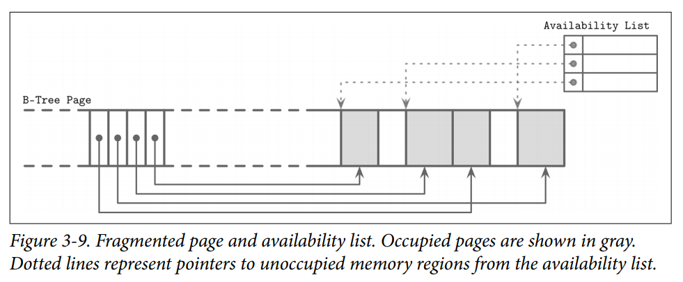
• Removing an item from the page does not have to remove the actual cell and shift other cells to reoccupy the freed space. Instead
  • the cell can be marked as deleted
  • an in-memory availability list can be updated with the amount of freed memory and a pointer to the freed value.
  • The availability list stores offsets of freed segments and their sizes. When inserting a new cell, we first check the availability list to find if there’s a segment where it may fit.
    
• Some database(Ex.SQLite) may store the the first available segments and total number of available bytes within the page to quickly check whether or not we can fit a new element into the page after defragmenting it.

Strategy to calculate fit

• First Fit: This might cause a larger overhead, since the space remaining after reusing the first suitable segment might be too small to fit any other cell, so it will be effectively wasted.
• Best Fit: For best fit, we try to find a segment for which insertion leaves the smallest remainder.

Others

• If we cannot find enough consecutive bytes to fit the new cell but there are enough fragmented bytes available, live cells are read and rewritten, defragmenting the page and reclaiming space for new writes. If there’s not enough free space even after defragmentation, we have to create an overflow page.
• To improve locality (especially when keys are small in size), some implementations store keys and values separately on the leaf level.Keeping keys together can improve the locality during the search. After the searched key is located, its value can be found in a value cell with a corresponding index. (Sorted) With variable-size keys, this requires us to calculate and store an additional value cell pointer

Summary

• In summary, to simplify B-Tree layout, we assume that each node occupies a single page. And a page consists of
  • fixed-size header
  • cell pointer block
  • cells
    • Cells hold keys and pointers to the pages representing child nodes or associated data records.
• BTrees use simple pointer hierarchies: page identifiers to locate the child nodes in the tree file, and cell offsets to locate cells within the page.

Versioning

The binary file format can change. Most of the time, any storage engine version has to support more than one serialization format. (e.g., current and one or more legacy formats for backward compatibility). To support that, we have to be able to find out which version of the file we’re up against.

• Apache Cassandra is using version prefixes in filenames. This way, you can tell which version the file has without even opening it. As of version 4.0, a data file name has the na prefix, such as na-1-bigData.db. Older files have different prefixes: files written in version 3.0 have the ma prefix.
• Alternatively, the version can be stored in a separate file. For example, PostgreSQL stores the version in the PG_VERSION file.
• The version can also be stored directly in the index file header. In this case, a part of the header (or an entire header) has to be encoded in a format that does not change between versions. After finding out which version the file is encoded with, we can create a version-specific reader to interpret the contents.

Checksumming

Files on disk may get damaged or corrupted by software bugs and hardware failures. To identify these problems preemptively and avoid propagating corrupt data to other subsystems or even nodes, we can use checksums and cyclic redundancy checks (CRCs).

• Checksums provide the weakest form of guarantee and aren’t able to detect corruption in multiple bits. They’re usually computed by using XOR with parity checks or summation.
• CRCs can help detect burst errors (e.g., when multiple consecutive bits got corrupted) and their implementations usually use lookup tables and polynomial division. Multibit errors are crucial to detect, since a significant percentage of failures in communication networks and storage devices manifest this way.

Noncryptographic hashes and CRCs should not be used to verify whether or not the data has been tampered with. For this, you should always use strong cryptographic hashes designed for security. The main goal of CRC is to make sure that there were no unintended and accidental changes in data. These algorithms are not designed to resist attacks and intentional changes in data

• Since computing a checksum over the whole file is often impractical and it is unlikely
  we’re going to read the entire content every time we access it, page checksums are
  usually computed on pages and placed in the page header. This way, checksums can
  be more robust (since they are performed on a small subset of the data), and the
  whole file doesn’t have to be discarded if corruption is contained in a single page

Implementing B-Trees

Page Header

• The page header holds information about the page that can be used for navigation, maintenance, and optimizations.
  • Flags that describe page contents and layout.
  • Number of cells in the page.
  • Lower and upper offsets marking the empty space (used to append cell offsets and data)
  • Other useful metadata
• PostgreSQL stores the page size and layout version in the header.
• MySQL InnoDB, page header holds the number of heap records, level, and some other implementation-specific values.
• In SQLite, page header stores the number of cells and a rightmost pointer.

Magic Numbers

One of the values often placed in the file or page header is a magic number. Usually, it’s a multibyte block, containing a constant value that can be used to signal that the block represents a page, specify its kind, or identify its version.

• Magic numbers are often used for validation and sanity checks. It’s
  very improbable that the byte sequence at a random offset would exactly match the magic number. If it did match, there’s a good chance the offset is correct.
  • Ex. during write we can place the magic number 50 41 47 45 (hex for PAGE) into the header. During the read, we validate the page by comparing the four bytes from the read header with the expected byte sequence.

Sibling Links

Some implementations store forward and backward links, pointing to the left and right sibling pages. These links help to locate neighboring nodes without having to ascend back to the parent. (One of differences between B-tree and B+Tree).

• Benefits: Range Query Performance
• Loss: Add complexity to split and merge operations as may need to update sibling offsets.

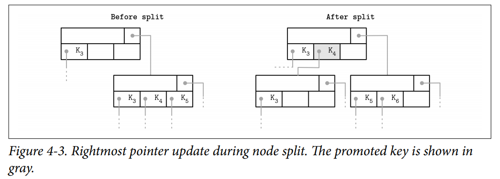
Rightmost Pointers

B-Tree separator keys have strict invariants: they’re used to split the tree into subtrees and navigate them, so there is always one more pointer to child pages than there are keys.

• In many implementations, nodes look more like the ones displayed in Figure 4-2: each separator key has a child pointer, while the last pointer is stored separately, since it’s not paired with any key. SQLite stored the extra pointer in the header.

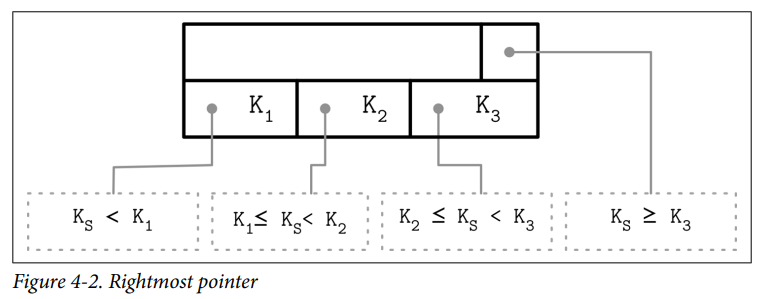
• If the rightmost child is split and the new cell is appended to its parent, the rightmost child pointer has to be reassigned. After the split, the cell appended to the parent (shown in gray) holds the promoted key and points to the split node. The pointer to the new node is assigned instead of the previous rightmost pointer.

Node High Keys