Database Internal - LSM-tree Summary

• The LSM-tree basic in database system.

• The LSM-tree basic in database system.
• Here is the basic of LSM-tree, including the knowledge of data structure and some optimization.
• The content is based on the book Database Internal. I will present my understanding.
• Only summary, not details.

Before LSM-tree

• Mutable Structures VS Immutable Structures
  • Mutable: In-place Update.
  • Immutable: Out-of-place Update
• In-place Update VS Out-of-place Update:
  • In-place update storage structures are optimized for read performance: after locating data on disk, the record can be returned to the client. This comes at the expense of write performance: to update the data record in place, it first has to be located on disk
  • Append-only storage is optimized for write performance. Writes do not have to locate records on disk to overwrite them. However, this is done at the expense of reads, which have to retrieve multiple data record versions and reconcile them.

Immutable Structures

• Safety characteristics: once created, an immutable structure doesn’t change, all of its references can be accessed concurrently, and its integrity is guaranteed by the fact that it cannot be modified.
• Immutable files can hold multiple copies, more recent ones overwriting the older ones, while mutable files generally hold only the most recent value instead.
• Immutable LSM Trees use append-only storage and merge reconciliationn, and B-Trees locate data records on disk and update pages at their original offsets in the file.

LSM-Tree

• We concluded that space overhead and write amplification can be improved by using buffering, and there are two ways buffering:
  • To postpone propagating writes to diskresident pages
  • To make write operations sequential.
• LSM Tree uses buffering and append-only storage to achieve sequential writes.
• LSM Trees defer data file writes and buffer changes in a memory-resident table.

LSM Structure

Two components

• Disk Components: Comprised of immutable segments and the disk component is organised as a B-tree, with 100% occupancy and read-only pages.
• Memory-resident tree contents are flushed on disk in parts. During a flush, for each flushed in-memory subtree, we find a corresponding subtree on disk and write out the merged contents of a memory-resident segment and disk-resident subtree into the new segment on disk.
  
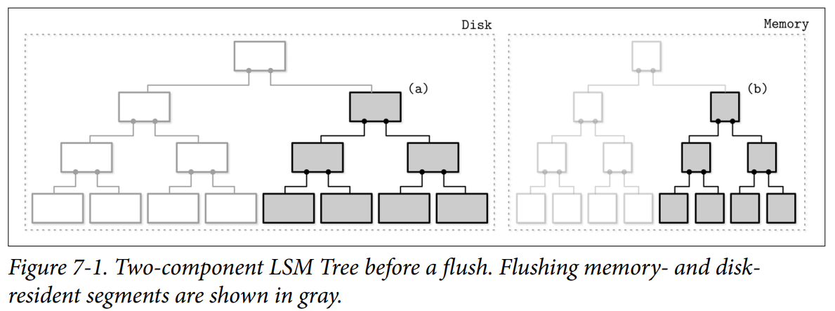
• After the subtree is flushed, superseded memory-resident and disk-resident subtrees are discarded and replaced with the result of their merge, which becomes addressable from the preexisting sections of the disk-resident tree.
  
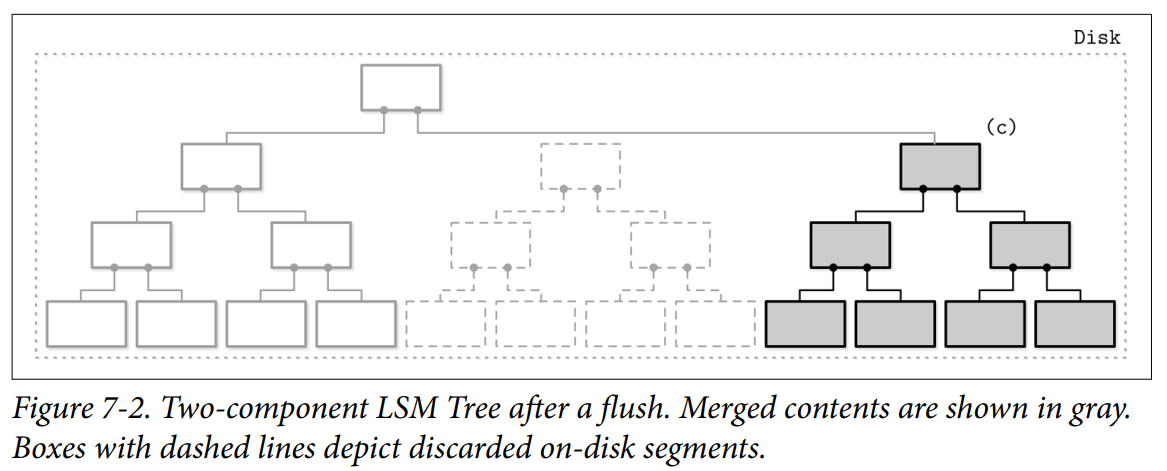
• A merge can be implemented by advancing iterators reading the disk-resident leaf nodes and contents of the in-memory tree in lockstep. Since both sources are sorted, to produce a sorted merged result, we only need to know the current values of both +iterators during each step of the merge process.
• This approach is a logical extension and continuation of our conversation on immutable B-Trees. Copy-on-write B-Trees use B-Tree structure, but their nodes are not fully occupied, and they require copying pages on the root-leaf path and creating a parallel tree structure. Here, we do something similar, but since we buffer writes in memory, we amortize the costs of the disk-resident tree update.
• As for merges and flushes:
  • As soon as the flush process starts, all new writes have to go to the new memtable. (Immutable Memtable and Mutable Memtable)
  • During the subtree flush, both the disk-resident and flushing memory-resident subtree have to remain accessible for reads.
  • Afer the flush, publishing merged contents, and discarding unmerged disk- and memory-resident contents have to be performed atomically.

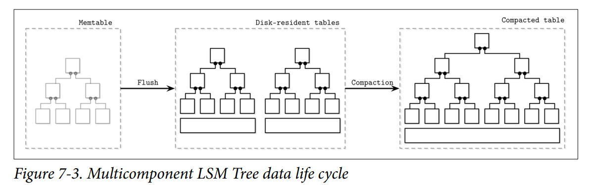
Multicomponent LSM Trees

Let’s consider an alternative design, multicomponent LSM Trees that have more than just one disk-resident table.

• It quickly becomes evident that after multiple flushes we’ll end up with multiple disk resident tables, and their number will only grow over time. Since we do not always know exactly which tables are holding required data records, we might have to access multiple files to locate the searched data.
• Having to read from multiple sources instead of just one might get expensive. To mitigate this problem and keep the number of tables to minimum, a periodic merge process called compaction is triggered.
• Compaction picks several tables, reads their contents, merges them, and writes the merged result out to the new combined file. Old tables are discarded simultaneously with the appearance of the new merged table.
  

In-memory Tables

• Flush Strategy: Memtable flushes can be triggered periodically, or by using a size threshold.

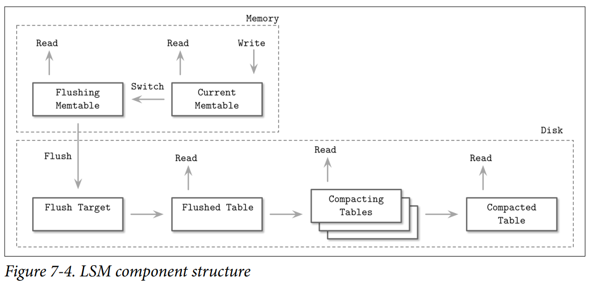
• Before memtable can be flushed, the memtable has to be switched: a new memtable is allocated, and it becomes a target for all new writes, while the old one moves to the flushing state. These two steps have to be performed atomically.

  • The flushing memtable remains available for reads until its contents are fully flushed.
  • After this, the old memtable is discarded in favor of a newly written disk-resident table, which becomes available for reads.

• Components

  • Current memtable: Receives writes and serves reads.
  • Flushing memtable: Available for reads.
  • On-disk flush target: Does not participate in reads, as its contents are incomplete.
  • Flushed tables: Available for reads as soon as the flushed memtable is discarded.
  • Compacting tables: Currently merging disk-resident tables.
  • Compacted tables: Created from flushed or other compacted tables.

Crash Consistency

Until the memtable is fully flushed, the only disk-resident version of its contents is stored in the write-ahead log. When memtable contents are fully flushed on disk, the log can be trimmed, and the log section, holding operations applied to the flushed memtable, can be discarded.

Updates And Deletes

• Core: Out-of-Place Updates

Delete

Single Key-Value

• Example: Delete k1
  
• Deletes need to be done by inserting a special delete entry (called tombstone or a dormant certificate) instead of removing directly.
  
• The reconciliation process picks up tombstones, and filters out the shadowed values.

Range Key-Value

• Sometimes it might be useful to remove a consecutive range of keys rather than just a single key. This can be done using predicate deletes, which work by appending a delete entry with a predicate that sorts according to regular record-sorting rules. During reconciliation, data records matching the predicate are skipped and not returned to the client. Such as DELETE FROM table WHERE key ≥ "k2" AND key < "k4".
• Apache Cassandra implements this approach and calls it range tombstones. A range tombstone covers a range of keys rather than just a single key.
• When using range tombstones, resolution rules have to be carefully considered because of overlapping ranges and disk-resident table boundaries.For example, the following combination will hide data records associated with k2 and k3 from the final result:
  

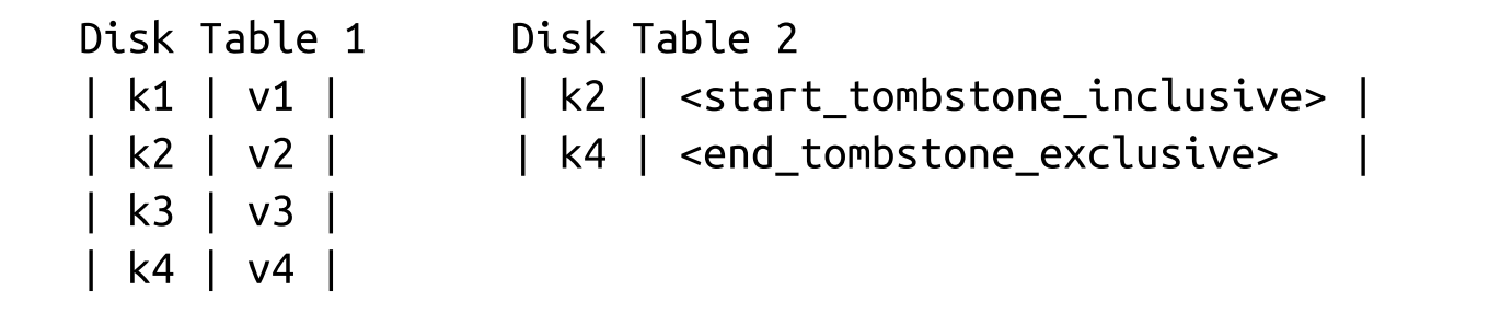
LSM Tree Lookups

LSM Trees consist of multiple components. During lookups, more than one component is usually accessed, so their contents have to be merged and reconciled before they can be returned to the client.

Merge-Iteration

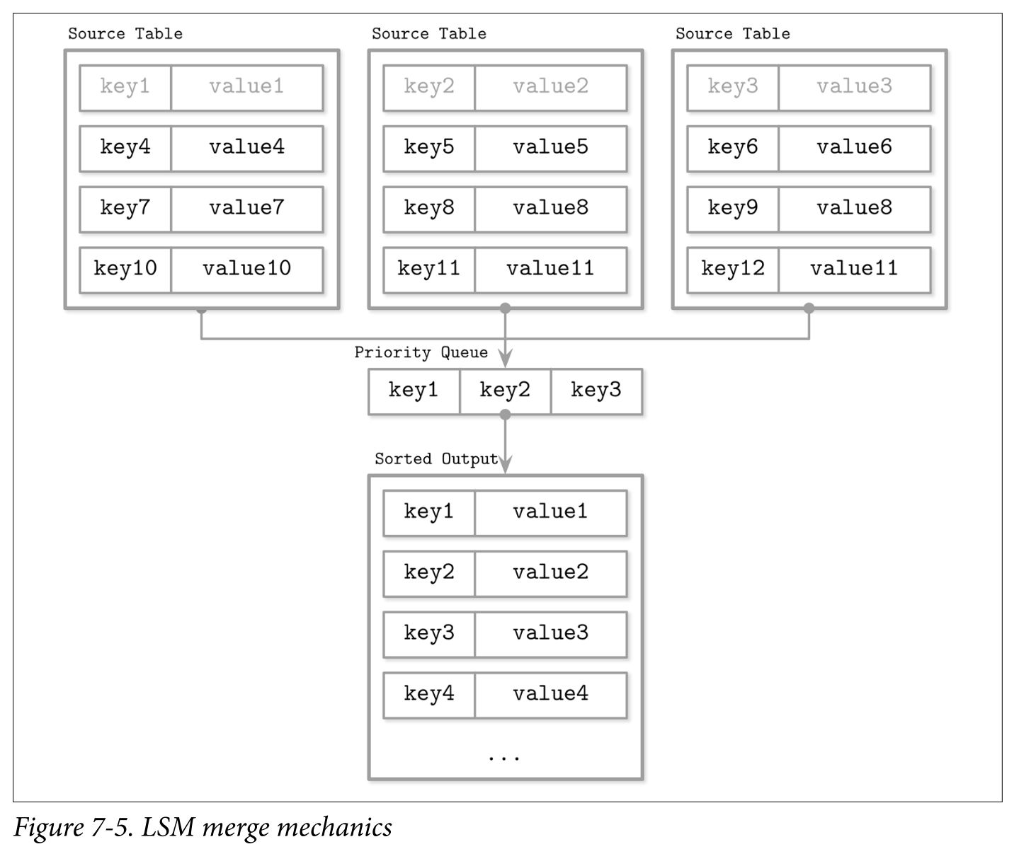
Since contents of disk-resident tables are sorted, we can use a multiway merge-sort algorithm.

• A multiway merge-sort uses a priority queue, such as min-heap that holds up to N elements (where N is the number of iterators), which sorts its contents and prepares the next-in-line smallest element to be returned. The head of each iterator is placed into the queue. An element in the head of the queue is then the minimum of all iterators.
• When the smallest element is removed from the queue, the iterator associated with it is checked for the next value, which is then placed into the queue, which is re-sorted to preserve the order.
• Since all iterator contents are sorted, reinserting a value from the iterator that held the previous smallest value of all iterator heads also preserves an invariant that the queue still holds the smallest elements from all iterators. Whenever one of the iterators is exhausted, the algorithm proceeds without reinserting the next iterator head. The algorithm continues until either query conditions are satisfied or all iterators are exhausted.

• It may happen that we encounter more than one data record for the same key during merge-iteration. From the priority queue and iterator invariants, we know that if each iterator only holds a single data record per key, and we end up with multiple records for the same key in the queue, these data records must have come from the different iterators.
• For example: two disk-resident tables:
  
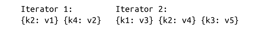
• The priority queue is filled from the iterator heads:
  
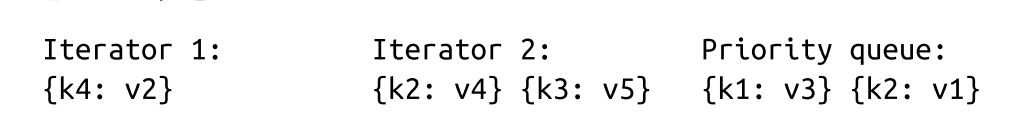
• Key k1 is the smallest key in the queue and is appended to the result. Since it came from Iterator 2, we refill the queue from it:
  
• Now, we have two records for the k2 key in the queue. We can be sure there are no other records with the same key in any iterator because of the aforementioned invariants. Same-key records are merged and appended to the merged result. The queue is refilled with data from both iterators:
  
• Since all iterators are now empty, we append the remaining queue contents to the output:
  

Steps:

1. Initially, fill the queue with the first items from each iterator.
2. Take the smallest element (head) from the queue.
3. Refill the queue from the corresponding iterator, unless this iterator is exhausted.

Overhead

In terms of complexity, merging iterators is the same as merging sorted collections. It has O(N) memory overhead, where N is the number of iterators. A sorted collection of iterator heads is maintained with O(log N) (average case)

Reconciliation

Merge-iteration is just a single aspect of what has to be done to merge data from multiple sources. Another important aspect is reconciliation and conflict resolution of the data records associated with the same key.

• To reconcile data records, we need to understand which one of them takes precedence. Data records hold metadata necessary for this, such as timestamps. To establish the order between the items coming from multiple sources and find out which one is more recent, we can compare their timestamps.
• Records shadowed by the records with higher timestamps are not returned to the client or written during compaction.

Maintenance in LSM Trees

• Compaction picks multiple disk-resident tables, iterates over their entire contents using the aforementioned merge and reconciliation algorithms, and writes out the results into the newly created table.
• Since disk-resident table contents are sorted, and because of the way merge-sort works, compaction has a theoretical memory usage upper bound, since it should only hold iterator heads in memory. All table contents are consumed sequentially, and the resulting merged data is also written out sequentially. These details may vary between implementations due to additional optimizations.
• Compacting tables remain available for reads until the compaction process finishes, which means that for the duration of compaction, it is required to have enough free space available on disk for a compacted table to be written.
• At any given time, multiple compactions can be executed in the system. However, these concurrent compactions usually work on nonintersecting sets of tables. A compaction writer can both merge several tables into one and partition one table into multiple tables.

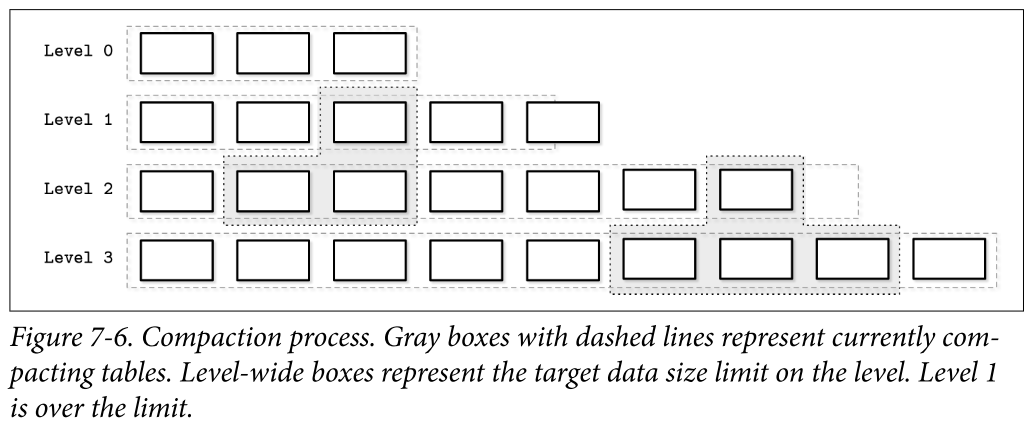
Leveled Compaction

One of the frequently implemented compaction strategies is called leveled compaction. For example, it is used by RocksDB.

• Leveled compaction separates disk-resident tables into levels. Tables on each level have target sizes, and each level has a corresponding index number (identifier).
• Level-0 tables are created by flushing memtable contents. Tables in level 0 may contain overlapping key ranges. As soon as the number of tables on level 0 reaches a threshold, their contents are merged, creating new tables for level 1.
• Key ranges for the tables on level 1 and all levels with a higher index do not overlap, so level-0 tables have to be partitioned during compaction, split into ranges, and merged with tables holding corresponding key ranges. Alternatively, compaction can include all level-0 and level-1 tables, and output partitioned level-1 tables.
• Compactions on the levels with the higher indexes pick tables from two consecutive levels with overlapping ranges and produce a new table on a higher level.

• Keeping different key ranges in the distinct tables reduces the number of tables accessed during the read. This is done by inspecting the table metadata and filtering out the tables whose ranges do not contain a searched key.
• Each level has a limit on the table size and the maximum number of tables. As soon as the number of tables on level 1 or any level with a higher index reaches a threshold, tables from the current level are merged with tables on the next level holding the overlapping key range.

Size-tiered compaction

In size-tiered compaction, rather than grouping disk-resident tables based on their level, they’re grouped by size: smaller tables are grouped with smaller ones, and bigger tables are grouped with bigger ones.

• Level 0 holds the smallest tables that were either flushed from memtables or created by the compaction process. When the tables are compacted, the resulting merged table is written to the level holding tables with corresponding sizes. The process continues recursively incrementing levels, compacting and promoting larger tables to higher levels, and demoting smaller tables to lower levels.

Read, Write, and Space Amplification

When implementing an optimal compaction strategy, we have to take multiple factors into consideration. One approach is to reclaim space occupied by duplicate records and reduce space overhead, which results in higher write amplification caused by rewriting tables continuously. The alternative is to avoid rewriting the data continuously, which increases read amplification (overhead from reconciling data records associated with the same key during the read), and space amplification (since redundant records are preserved for a longer time).

• Read amplification：Resulting from a need to address multiple tables to retrieve data.
• Write amplification：Caused by continuous rewrites by the compaction process.
• Space amplification：Arising from storing multiple records associated with the same key.

Implementation Details

• how memory- and disk-resident tables are implemented
• how secondary indexes work
• how to reduce the number of diskresident tables accessed during read and
• new ideas related to log-structured storage.

Sorted String Tables

Disk-resident tables are often implemented using Sorted String Tables (SSTables). As the name suggests, data records in SSTables are sorted and laid out in key order.

• SSTables usually consist of two components: index files and data files.

Index files

• Index files are implemented using some structure allowing logarithmic lookups, such as B-Trees, or constant-time lookups, such as hashtables.
• The index component holds keys and data entries (offsets in the data file where the actual data records are located).

Data files

• The data component consists of concatenated key-value pairs.
• The cell design and data record formats we discussed in Chapter 3 are largely applicable to SSTables. The main difference here is that cells are written sequentially and are not modified during the life cycle of the SSTable. Since the index files hold pointers to the data records stored in the data file, their offsets have to be known by the time the index is created.
• During compaction, data files can be read sequentially without addressing the index component, as data records in them are already ordered. Since tables merged during compaction have the same order, and merge-iteration is order-preserving, the resulting merged table is also created by writing data records sequentially in a single run. As soon as the file is fully written, it is considered immutable, and its disk-resident contents are not modified.

SSTable-Attached Secondary Indexes

• Apache Cassandra： SSTableAttached Secondary Indexes (SASI)
  • To allow indexing table contents not just by the primary key, but also by any other field, index structures and their life cycles are coupled with the SSTable life cycle, and an index is created per SSTable.
  • When the memtable is flushed, its contents are written to disk, and secondary index files are created along with the SSTable primary key index.
• Since LSM Trees buffer data in memory and indexes have to work for memory-resident contents as well as the disk-resident ones, SASI maintains a separate in-memory structure, indexing memtable contents.

Bloom Filters

• One of the ways to prevent table lookup is to store its key range (smallest and largest keys stored in the given table) in metadata, and check if the searched key belongs to the range of that table. This information is imprecise and can only tell us if the data record can be present in the table. To improve this situation, many implementations, including Apache Cassandra and RocksDB, use a data structure called a Bloom filter.
• Bloom filter can be used to tell if the key might be in the table or is definitely not in the table. Using Bloom filters associated with disk-resident tables helps to significantly reduce the number of tables accessed during a read.
• More details please visit Bloom Filters;

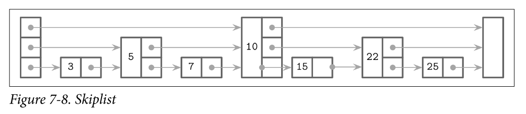
Skiplist

• There are many different data structures for keeping sorted data in memory, and one that has been getting more popular recently because of its simplicity is called a skiplist
• Skiplists do not require rotation or relocation for inserts and updates, and use probabilistic balancing instead. Skiplists are generally less cache-friendly than in-memory B-Trees, since skiplist nodes are small and randomly allocated in memory. Some implementations improve the situation by using unrolled linked lists.
• A skiplist consists of a series of nodes of a different height, building linked hierarchies allowing to skip ranges of items. Each node holds a key, and, unlike the nodes in a linked list, some nodes have more than just one successor. A node of height h is linked from one or more predecessor nodes of a height up to h. Nodes on the lowest level can be linked from nodes of any height.
• Node height is determined by a random function and is computed during insert. Nodes that have the same height form a level. The number of levels is capped to avoid infinite growth, and a maximum height is chosen based on how many items can be held by the structure. There are exponentially fewer nodes on each next level.
• Lookups work by following the node pointers on the highest level. As soon as the search encounters the node that holds a key that is greater than the searched one, its predecessor’s link to the node on the next level is followed. In other words, if the searched key is greater than the current node key, the search continues forward. If the searched key is smaller than the current node key, the search continues from the predecessor node on the next level. This process is repeated recursively until the searched key or its predecessor is located.

Lookup Example

• Searching for key 7 in the skiplist
  • Follow the pointer on the highest level, to the node that holds key 10. 7 < 10
  • Since the searched key 7 is smaller than 10, the next-level pointer from the head node is followed, locating a node holding key 5. 7 > 5
  • The highest-level pointer on this node is followed, locating the node holding key 10 again. 7 < 10
  • The searched key 7 is smaller than 10, and the next-level pointer from the node holding key 5 is followed, locating a node holding the searched key 7.

Insert

• During insert, an insertion point (node holding a key or its predecessor) is found using the aforementioned algorithm, and a new node is created. To build a tree-like hierarchy and keep balance, the height of the node is determined using a random number, generated based on a probability distribution.
• Pointers in predecessor nodes holding keys smaller than the key in a newly created node are linked to point to that node. Their higher-level pointers remain intact. Pointers in the newly created node are linked to corresponding successors on each level.

Delete

• orward pointers of the removed node are placed to predecessor nodes on corresponding levels.

Other

• We can create a concurrent version of a skiplist by implementing a linearizability scheme that uses an additional fully_linked flag that determines whether or not the node pointers are fully updated. This flag can be set using compare-and-swap. This is required because the node pointers have to be updated on multiple levels to fully restore the skiplist structure
• In languages with an unmanaged memory model, reference counting or hazard pointers can be used to ensure that currently referenced nodes are not freed while they are accessed concurrently. This algorithm is deadlock-free, since nodes are always accessed from higher levels.
• Apache Cassandra uses skiplists for the secondary index memtable implementation. WiredTiger uses skiplists for some in-memory operations.
• SkipList Details

Disk Access

• Since most of the table contents are disk-resident, and storage devices generally allow accessing data blockwise, many LSM Tree implementations rely on the page cache for disk accesses and intermediate caching. Many techniques described in “Buffer Management” on page 81, such as page eviction and pinning, still apply to log-structured storage.
• The most notable difference is that in-memory contents are immutable and therefore require no additional locks or latches for concurrent access. Reference counting is applied to make sure that currently accessed pages are not evicted from memory, and in-flight requests complete before underlying files are removed during compaction.
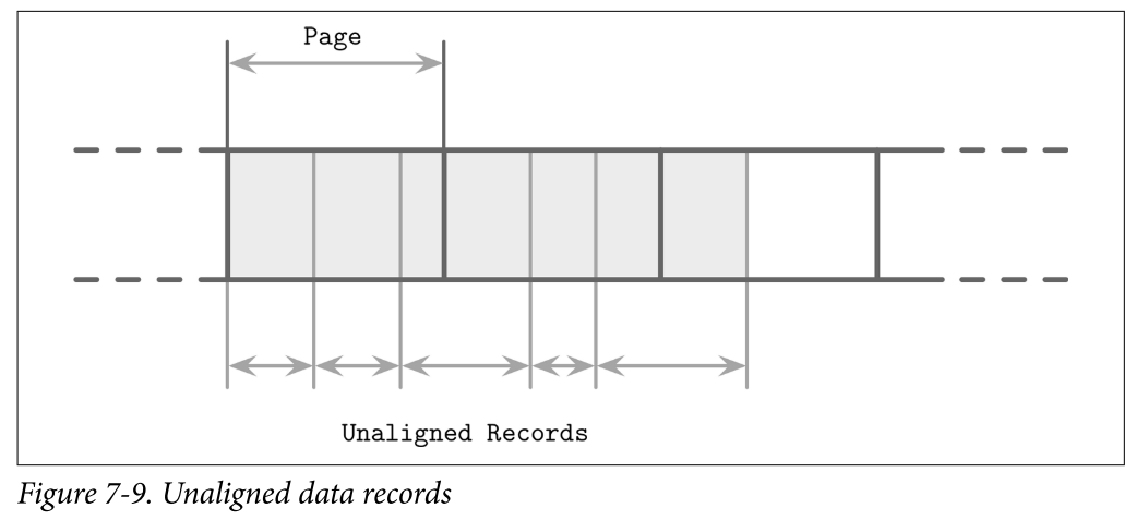
• Another difference is that data records in LSM Trees are not necessarily page aligned, and pointers can be implemented using absolute offsets rather than page IDs for addressing. In Figure 7-9, you can see records with contents that are not aligned with disk blocks. Some records cross the page boundaries and require loading several pages in memory.
  

Compression

• We’ve discussed compression already in context of B-Trees. Similar ideas are also applicable to LSM Trees. The main difference here is that LSM Tree tables are immutable, and are generally written in a single pass. When compressing data page-wise, compressed pages are not page aligned, as their sizes are smaller than that of uncompressed ones.
• To be able to address compressed pages, we need to keep track of the address boundaries when writing their contents. We could fill compressed pages with zeros, aligning them to the page size, but then we’d lose the benefits of compression.
• To make compressed pages addressable, we need an indirection layer which stores offsets and sizes of compressed pages. Figure 7-10 shows the mapping between compressed and uncompressed blocks. Compressed pages are always smaller than the originals, since otherwise there’s no point in compressing them.
  
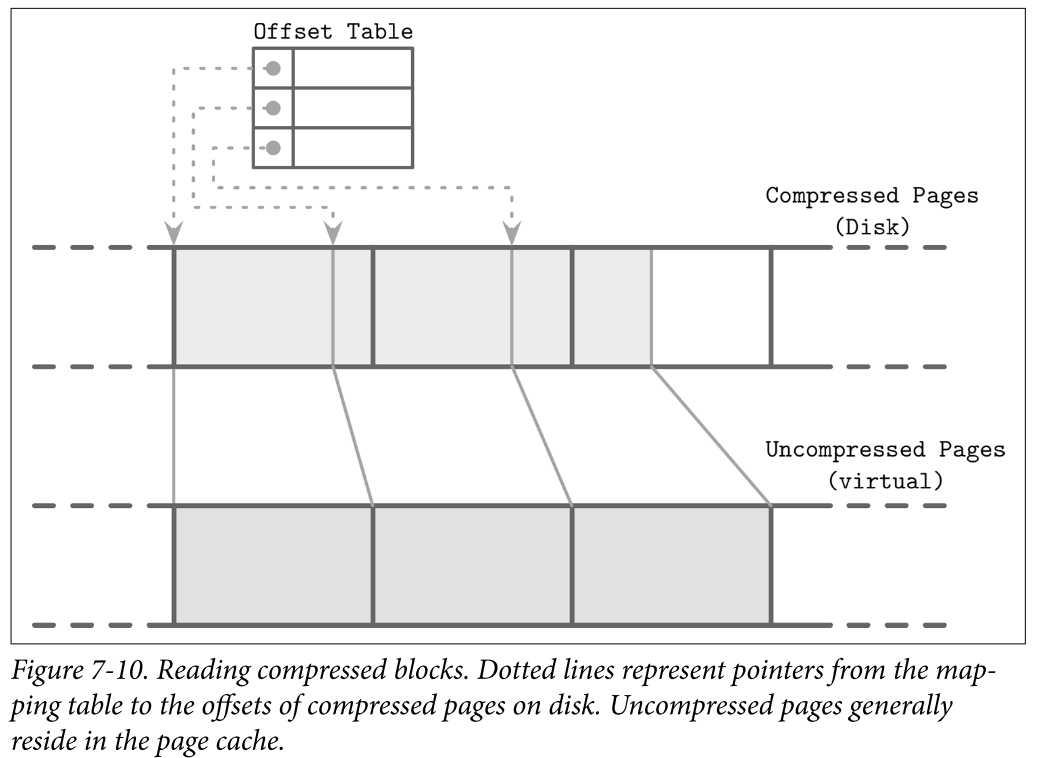
• During compaction and flush, compressed pages are appended sequentially, and compression information (the original uncompressed page offset and the actual compressed page offset) is stored in a separate file segment. During the read, the compressed page offset and its size are looked up, and the page can be uncompressed and materialized in memory.

Unordered LSM Storage

Unordered stores generally do not require a separate log and allow us to reduce the cost of writes by storing data records in insertion order.

Bitcask

Bitcask, one of the storage engines used in Riak, is an unordered log-structured storage engine. Unlike the log-structured storage implementations discussed so far, it does not use memtables for buffering, and stores data records directly in logfiles.

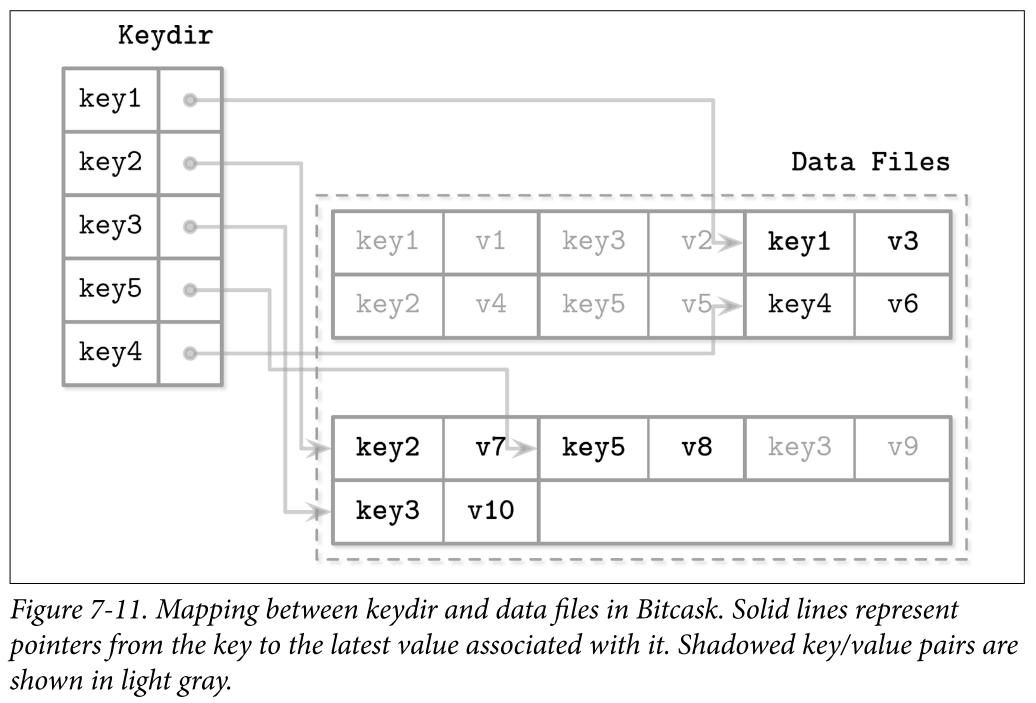
• To make values searchable, Bitcask uses a data structure called keydir, which holds references to the latest data records for the corresponding keys. Old data records may still be present on disk, but are not referenced from keydir, and are garbage-collected during compaction. Keydir is implemented as an in-memory hashmap and has to be rebuilt from the logfiles during startup.
  • Write: During a write, a key and a data record are appended to the logfile sequentially, and the pointer to the newly written data record location is placed in keydir.
  • Read: Reads check the keydir to locate the searched key and follow the associated pointer to the logfile, locating the data record. Since at any given moment there can be only one value associated with the key in the keydir, point queries do not have to merge data from multiple sources. Figure 7-11 shows mapping between the keys and records in data files in Bitcask. Logfiles hold data records, and keydir points to the latest live data record associated with each key. Shadowed records in data files (ones that were superseded by later writes or deletes) are shown in gray.
    
  • Compaction: During compaction, contents of all logfiles are read sequentially, merged, and written to a new location, preserving only live data records and discarding the shadowed ones. Keydir is updated with new pointers to relocated data records.
• Data records are stored directly in logfiles, so a separate write-ahead log doesn’t have to be maintained, which reduces both space overhead and write amplification. A downside of this approach is that it offers only point queries and doesn’t allow range scans, since items are unordered both in keydir and in data files.

Benefits and Disadvantages

• Advantages of this approach are simplicity and great point query performance. Even though multiple versions of data records exist, only the latest one is addressed by keydir.
• However, having to keep all keys in memory and rebuilding keydir on startup are limitations that might be a deal breaker for some use cases.
• While this approach is great for point queries, it does not offer any support for range queries.

WiscKey

WiscKey decouples sorting from garbage collection by keeping the keys sorted in LSM Trees, and keeping data records in unordered append-only files called vLogs (value logs). This approach can solve two problems mentioned while discussing Bitcask: a need to keep all keys in memory and to rebuild a hashtable on startup.

• Figure 7-12 shows key components of WiscKey, and mapping between keys and log files. vLog files hold unordered data records. Keys are stored in sorted LSM Trees, pointing to the latest data records in the logfiles.
  
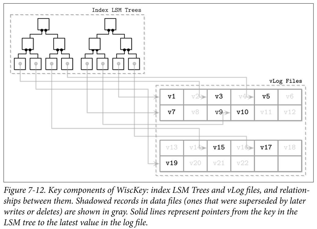
• Since keys are typically much smaller than the data records associated with them, compacting them is significantly more efficient. This approach can be particularly useful for use cases with a low rate of updates and deletes, where garbage collection won’t free up as much disk space.
• The main challenge here is that because vLog data is unsorted, range scans require random I/O. WiscKey uses internal SSD parallelism to prefetch blocks in parallel during range scans and reduce random I/O costs. In terms of block transfers, the costs are still high: to fetch a single data record during the range scan, the entire page where it is located has to be read.
• During compaction, vLog file contents are read sequentially, merged, and written to a new location. Pointers (values in a key LSM Tree) are updated to point to these new locations. To avoid scanning entire vLog contents, WiscKey uses head and tail pointers, holding information about vLog segments that hold live keys.
• Since data in vLog is unsorted and contains no liveness information, the key tree has to be scanned to find which values are still live. Performing these checks during garbage collection introduces additional complexity: traditional LSM Trees can resolve file contents during compaction without addressing the key index.
• More details please visist WiscKey in my Blog

Concurrency in LSM Trees

• The main concurrency challenges in LSM Trees are related to switching table views (collections of memory- and disk-resident tables that change during flush and compaction) and log synchronization. Memtables are also generally accessed concurrently (except core-partitioned stores such as ScyllaDB), but concurrent in-memory data structures are out of the scope of this book.

Flush Rules

• The new memtable has to become available for reads and writes.
• The old (flushing) memtable has to remain visible for reads.
• The flushing memtable has to be written on disk.
• Discarding a flushed memtable and making a flushed disk-resident table have to be performed as an atomic operation.
• The write-ahead log segment, holding log entries of operations applied to the flushed memtable, has to be discarded.

Approaches

• Apache Cassandra solves these problems by using operation order barriers: all operations that were accepted for write will be waited upon prior to the memtable flush. This way the flush process (serving as a consumer) knows which other processes (acting as producers) depend on it.

Synchronization points

• Memtable switch: After this, all writes go only to the new memtable, making it primary, while the old one is still available for reads.
• Flush finalization: Replaces the old memtable with a flushed disk-resident table in the table view.
• Write-ahead log truncation: Discards a log segment holding records associated with a flushed memtable.

Log Stacking

• Many modern filesystems are log structured: they buffer writes in a memory segment and flush its contents on disk when it becomes full in an append-only manner
• SSDs use log-structured storage, too, to deal with small random writes, minimize write overhead, improve wear leveling, and increase device lifetime.
• LSM Trees and SSDs are a good match, since sequential workloads and append-only writes help to reduce amplification from inplace updates, which negatively affect performance on SSDs.
• If we stack multiple log-structured systems on top each other, we can run into several problems that we were trying to solve using LSS, including write amplification, fragmentation, and poor performance. At the very least, we need to keep the SSD flash translation layer and the filesystem in mind when developing our applications

FTL Flash Translation Layer

• Using a log-structuring mapping layer in SSDs is motivated by two factors:
  • small random writes have to be batched together in a physical page
  • the fact that SSDs work by using program/erase cycles.
• Writes can be done only into previously erased pages. This means that a page cannot be programmed (in other words, written) unless it is empty (in other words, was erased).
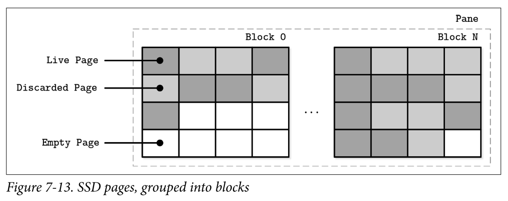
• A single page cannot be erased, and only groups of pages in a block (typically holding 64 to 512 pages) can be erased together. Figure 7-13 shows a schematic representation of pages, grouped into blocks. The flash translation layer (FTL) translates logical page addresses to their physical locations and keeps track of page states (live, discarded, or empty). When FTL runs out of free pages, it has to perform garbage collection and erase discarded pages.
  
• There are no guarantees that all pages in the block that is about to be erased are discarded. Before the block can be erased, FTL has to relocate its live pages to one of the blocks containing empty pages. Figure 7-14 shows the process of moving live pages from one block to new locations.
  
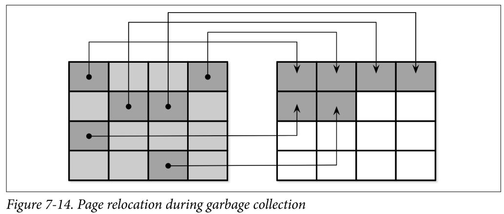
• When all live pages are relocated, the block can be safely erased, and its empty pages become available for writes. Since FTL is aware of page states and state transitions and has all the necessary information, it is also responsible for SSD wear leveling.

Wear leveling distributes the load evenly across the medium, avoiding hotspots, where blocks fail prematurely because of a high number of program-erase cycles. It is required, since flash memory cells can go through only a limited number of program-erase cycles, and using memory cells evenly helps to extend the lifetime of the device.

Summary

• In summary, the motivation for using log-structured storage on SSDs is to amortize I/O costs by batching small random writes together, which generally results in a smaller number of operations and, subsequently, reduces the number of times the garbage collection is triggered.

Filesystem Logging

On top of that, we get filesystems, many of which also use logging techniques for write buffering to reduce write amplification and use the underlying hardware optimally.

• Log stacking manifests in a few different ways. First, each layer has to perform its own bookkeeping, and most often the underlying log does not expose the information necessary to avoid duplicating the efforts.
• Figure 7-15 shows a mapping between a higher-level log (for example, the application) and a lower-level log (for example, the filesystem) resulting in redundant logging and different garbage collection patterns. Misaligned segment writes can make the situation even worse, since discarding a higher-level log segment may cause fragmentation and relocation of the neighboring segments’ parts.
  
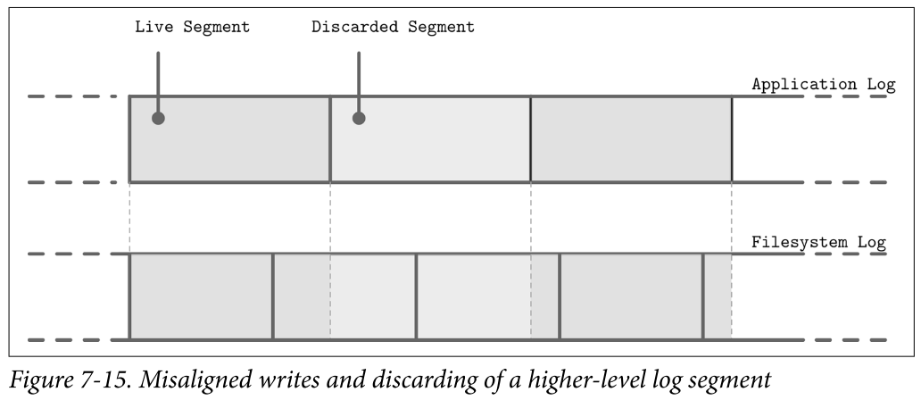
• Because layers do not communicate LSS-related scheduling (for example, discarding or relocating segments), lower-level subsystems might perform redundant operations on discarded data or the data that is about to be discarded. Similarly, because there’s no single, standard segment size, it may happen that unaligned higher-level segments occupy multiple lower-level segments. All these overheads can be reduced or completely avoided.
• Even though we say that log-structured storage is all about sequential I/O, we have to keep in mind that database systems may have multiple write streams (for example, log writes parallel to data record writes). When considered on a hardware level, interleaved sequential write streams may not translate into the same sequential pattern: blocks are not necessarily going to be placed in write order. Figure 7-16 shows multiple streams overlapping in time, writing records that have sizes not aligned with the underlying hardware page size.
  
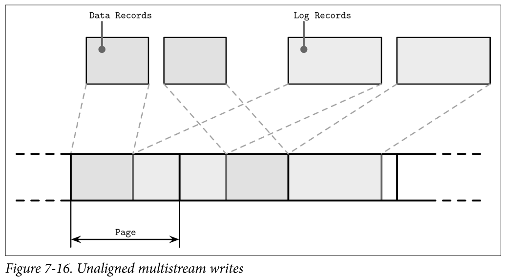
• This results in fragmentation that we tried to avoid. To reduce interleaving, some database vendors recommend keeping the log on a separate device to isolate workloads and be able to reason about their performance and access patterns independently. However, it is more important to keep partitions aligned to the underlying hardware and keep writes aligned to page size.

LLAMA and Mindful Stacking

Bw-Tree is layered on top of a latch-free, log-structured, access-method aware (LLAMA) storage subsystem. This layering allows Bw-Trees to grow and shrink dynamically, while leaving garbage collection and page management transparent for the tree. Here, we’re most interested in the access-method aware part, demonstrating the benefits of coordination between the software layers.

• Without access-method awareness, interleaved delta nodes that belong to different logical nodes will be written in their insertion order. Bw-Tree awareness in LLAMA allows for the consolidation of several delta nodes into a single contiguous physical location. If two updates in delta nodes cancel each other (for example, an insert followed by delete), their logical consolidation can be performed as well, and only the latter delete can be persisted.
• LSS garbage collection can also take care of consolidating the logical Bw-Tree node contents. This means that garbage collection will not only reclaim the free space, but also significantly reduce the physical node fragmentation. If garbage collection only rewrote several delta nodes contiguously, they would still take the same amount of space, and readers would need to perform the work of applying the delta updates to the base node. At the same time, if a higher-level system consolidated the nodes and wrote them contiguously to the new locations, LSS would still have to garbage-collect the old versions.
• By being aware of Bw-Tree semantics, several deltas may be rewritten as a single base node with all deltas already applied during garbage collection. This reduces the total space used to represent this Bw-Tree node and the latency required to read the page while reclaiming the space occupied by discarded pages.
• You can see that, when considered carefully, stacking can yield many benefits. It is not necessary to always build tightly coupled single-level structures. Good APIs and exposing the right information can significantly improve efficiency.

Open-Channel SSDs

An alternative to stacking software layers is to skip all indirection layers and use the
hardware directly. For example, it is possible to avoid using a filesystem and flash translation layer by developing for Open-Channel SSDs.

• This way, we can avoid at least two layers of logs and have more control over wear-leveling, garbage collection, data placement, and scheduling.
  • One of the implementations that uses this approach is LOCS (LSM Tree-based KV Store on Open-Channel SSD)
    • Wang, Peng, Guangyu Sun, Song Jiang, Jian Ouyang, Shiding Lin, Chen Zhang, and Jason Cong. 2014. “An Efficient Design and Implementation of LSM-tree based Key-Value Store on Open-Channel SSD.” EuroSys ’14 Proceedings of the Ninth European Conference on Computer Systems (April): Article 16. https://doi.org/10.1145/2592798.2592804.
  • Another example using Open-Channel SSDs is LightNVM, implemented in the Linux kernel
    • Bjørling, Matias, Javier González, and Philippe Bonnet. 2017. “LightNVM: the Linux open-channel SSD subsystem.” In Proceedings of the 15th Usenix Conference on File and Storage Technologies (FAST’17), 359-373. USENIX.
• You can draw a parallel with using the O_DIRECT flag to bypass the kernel page cache, which gives better control, but requires manual page management.
• Software Defined Flash (SDF) [OUYANG14 SDF: software-defined flash for web-scale internet storage systems.”], a hardware/software codesigned OpenChannel SSDs system, exposes an asymmetric I/O interface that takes SSD specifics into consideration.
  • Sizes of read and write units are different, and write unit size corresponds to erase unit size (block), which greatly reduces write amplification. This setting is ideal for log-structured storage, since there’s only one software layer that performs garbage collection and relocates pages.
  • Additionally, developers have access to internal SSD parallelism, since every channel in SDF is exposed as a separate block device, which can be used to further improve performance.
• Hiding complexity behind a simple API might sound compelling, but can cause complications in cases in which software layers have different semantics. Exposing some underlying system internals may be beneficial for better integration.

Summary

• Log-structured storage is used everywhere: from the flash translation layer, to filesystems and database systems. It helps to reduce write amplification by batching small random writes together in memory. To reclaim space occupied by removed segments, LSS periodically triggers garbage collection.
• LSM Trees take some ideas from LSS and help to build index structures managed in a log-structured manner: writes are batched in memory and flushed on disk; shadowed data records are cleaned up during compaction.
• It is important to remember that many software layers use LSS, and make sure that layers are stacked optimally. Alternatively, we can skip the filesystem level altogether and access hardware directly